SDT-base         Contents     Functions              PDF Index

2.7  Identification by block

• Data format
• Tutorial

Previous sections have focused on the identification of SIMO or MIMO transfers. For some test cases, it is necessary to perform several identification by blocks because pole shifts are expected between these blocks. Here are examples of typical parameters defining the blocks :

• Temperature
• Input location
• Input level
• Pre-loading
• ...

The IdentBy strategy provides tools to easily navigate between blocks, perfom the identification for each block and finally post-treat the result (pole tracking, clustering, main shape extraction,...)

2.7.1  Data format

Section 2.2.5 explains how to store transfers in the Multi-dim curve format. The IdentBy strategy also uses this format. When only one parameter is used to identify the blocks (temperature ot input number for instance), you must build your curve structure with filed in this order : Frequencies, outputs, inputs and finally the block parameter (note that if the parameter correponds to the inputs, you do not need a fourth dimension).

An example of measurement with blocks depending on the temperature is given in demo. The following script stores the measurements in iiplot and initializes the IdentBy procedure

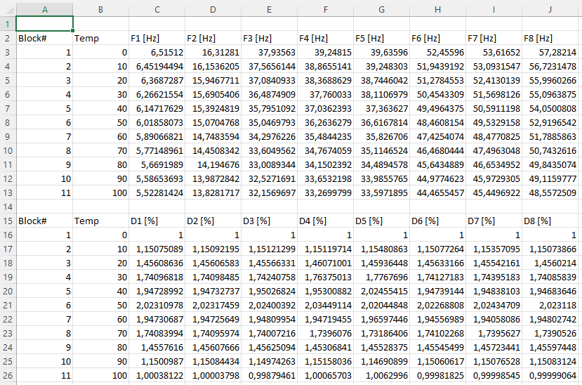
[XF,wire]=demosdt('DemoGartBy');
[ci,cf]=iicom('dockid',struct('model',wire,'XF',XF)); % Open dock with measurement blocks in curve 'Test'
idcom(ci,'ByInitFromTest'); % Same as click on button InitByMode
ci.Stack{'Test:All'}.By % Display the range structure defining the block

In the example above, the curve contains 4 dimension with

• 691 frequency samples
• 24 outputs
• 3 inputs
• 11 temperature samples (this is our block parameter)

The command idcom(ci,'ByInitFromTest'); has automatically created a range structure (see fe_range) stored in the field .By of curve 'Test:All' that defines each experiment block. This automatic range definition works for simple measurement blocks : only the last curve dimension is considered as the block parameter. For more complex configurations with several block parameters, you need to build the rangestructure yourself and eventually the doSplit strategy (how to extract a single block from Test:All curve).

2.7.2  Tutorial

The following tutorial highlights the use of the IdentBy procedure through the identification of the DemoGartBy example.

1. Run Load the curve containing all the measurement blocks and eventually the wireframe. Store them in the dock Id with the command

   [XF,wire]=demosdt('DemoGartBy'); % Example of measurement blocks with GARTEUR
   [ci,cf]=iicom('dockid',struct('model',wire,'XF',XF)); % Open dock with measurement blocks in curve 'Test'
   

   

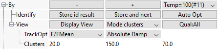
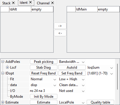
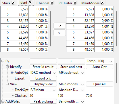
2. Run To initialize the identification by block, activate tab Ident, expand IDopt and click on Init By Mode.

   In the Ident tab, a block of buttons By has appeared.

   

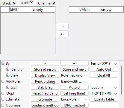
   These buttons help in the navigation between block through the whole procedure of identification by blocks. All the blocks are listed in the pop button on the top right (here 11 temperatures). You can increase or decrease the selected block by clicking on the + or - buttons or directly selecting the wanted one in the list. When one block is selected, measurement data corresponding to this block only is stored in the curve Test and eventually the synthesized transfer (if previous identification has been performed).

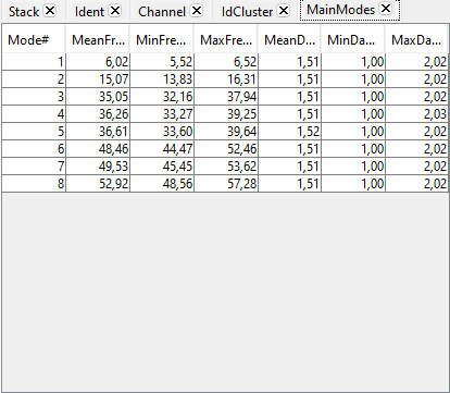
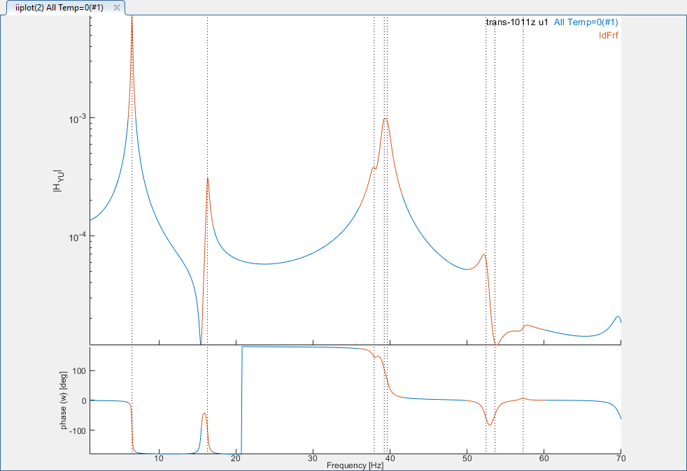
3. Run To initialize the procedure, select the first block and classically perform the identification: add poles and estimate transfers using LocalPole strategy.

   To speed up, you can manually add this list of poles :

    ci.Stack{'IdMain'}.po=[
    %{'Freq','Damp','Index'}
     6.51512 0.010000 % 1 
    16.31281 0.010000 % 2 
    37.93563 0.010000 % 3 
    39.24815 0.010000 % 4 
    39.63596 0.010000 % 5 
    52.45596 0.010000 % 6 
    53.61652 0.010000 % 7 
    57.28214 0.010000 % 8 
    ];
    ci.Stack{'IdMain'}.BandType='LocalPole';
    iicom('SetIdent',struct('est','do'));
   

   

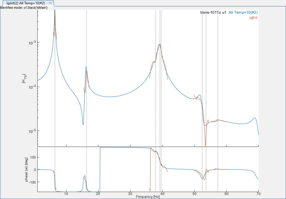
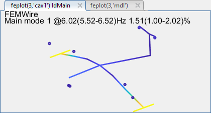
4. Run Once the identification of the first block is satisfying, store the result by clicking on Store and Next. The button callback stores the poles of the first block of transfers and load the second block of transfers while keeping the poles.

   Click on Estimate to perform estimation with these poles. The result is not good because at this new temperature, the poles have slightly evolve.

   

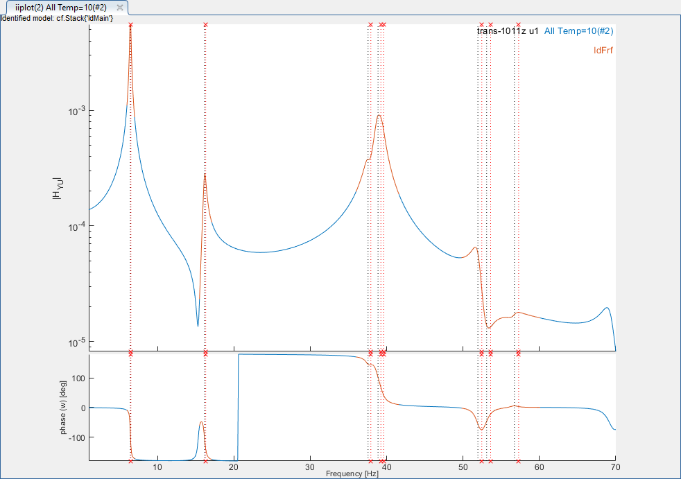
5. Run Optimize the poles using for instance IDRC method.

   Poles converge toward a satisying result.

   Save this result in the current block with the button Store.

   

6. Run Rather than manually optimizing poles between consecutive blocks on transfers, automatic optimization can be performes by clicking on button Auto Opt.

   Wait for the automatic optimization to end.

   If for some reason, the optimzation fails of diverges, it is possible to manually come back to the problematic block of transfer, modifiy identification and restart optimization procedure from there.

7. Run Now that poles of all transfer blocks are identified, it is possible to analyze the result using SDT tools or export the result in a spreadsheet (Excel) for custom analysis.

   Under By, Identify, AutoOpt, click on Export .xls to generate the Excel spreadsheet.

   

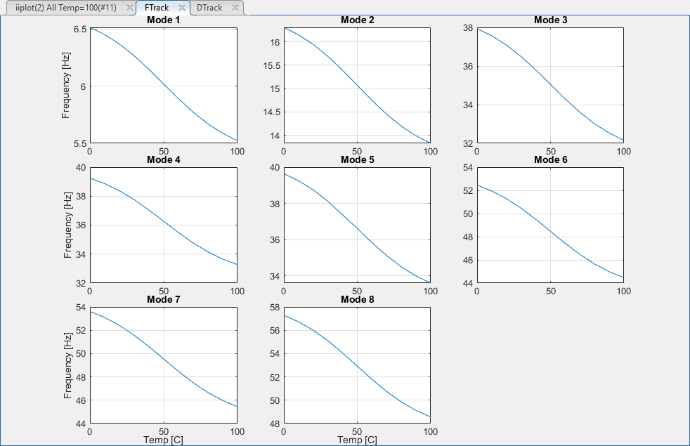
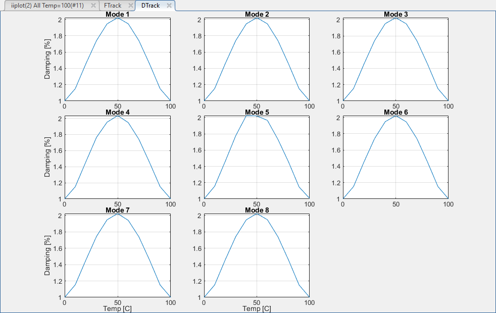
8. Run Pole tracking with parameter (here temperature) can be analyze with SDT views. In tab Ident, at line Identify, select Pole Tracking and click on View.

   This opens the two figures showing frequency and damping evolution of each mode with temperature.

   

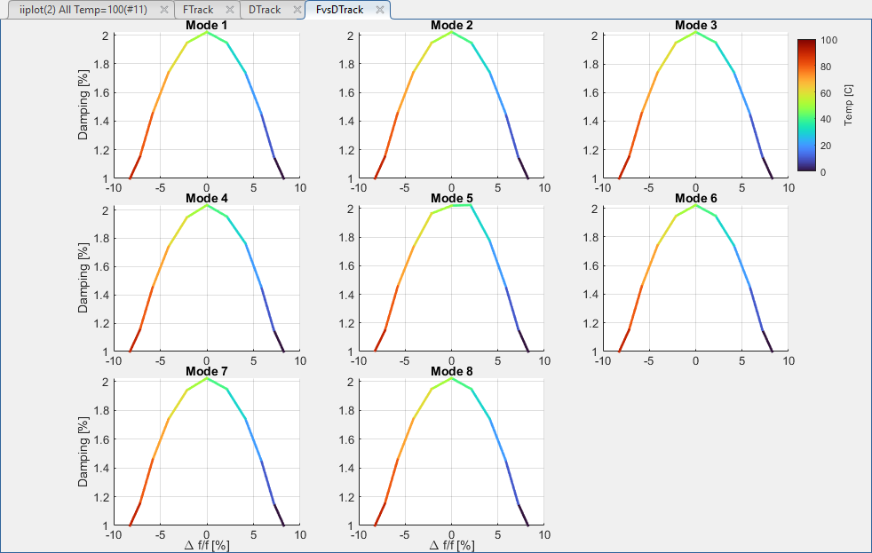
9. Run Both frequency and damping evolution with temperature can be displayed all at once. Select Pole Tracking fvsd and click on View.

   This opens the figure showing frequency (x-axis) and damping (y-axis) evolution of each mode with temperature (color).

   

10. Run This recent step is here for reference but not documented yet.

    

11. Run This recent step is here for reference but not documented yet.